This self-created algorithm was done to avoid the lack of standardization of the data and the poor impact of the most valued variable. The algorithm is based on evaluating variables according to their performance and impact on the target variable, as well as their relative impact on all the different variables. To evaluate the variables, the algorithm will return a value between -1 and 2, where -1 will be assigned to the variable with the worst performance and 2 to the best. Once all the variables are evaluated, we will take the average of them to obtain the “final_technical_value,” which represents a technical value indicating how likely that set of variables will achieve the expected target variable. To explain this algorithm, I think it is easy to do so with an example:
Example
We are going to use the RM algorithm to predict the math grade of Michel. We will use the grades of 15 subjects to predict the math grade. Imagine we have a historical dataset with 200k students, including the grades of the fifteen subjects and the math grades, which will be our target variable.
Explanation step by step: To study how correlated the grades of other subjects are with the math grade, we are going to analyze the students based on their performance in other subjects and compare it to the math grade. We will start with an example of how the grades of physics are correlated with the math grade.
1. Group the students according to the performance:
The first step is to group the students by how they perform in physics so we can see trends and how correlated are the two subjects in a global way. How to group the students ?
– The students that got an 7,8 or higher in physics are in the top 25% with better grades, this group will be named GROUP 1.
– The students that got a grade between 7,8 and 4,3 that is the 50% of the class would be in the middle ( The persons that perform better than the 25% worse but less than the 25% higher. This will be the GROUP 2.
– The students with less than 4,3 would be in the group 3, because they are in the 25% worse performance. This will be the GROUP 3.
– Finally, the GROUP 4 would be all the persons that didn’t do physics, the not rated or there is no data.
2. Studying the groups:
Once we got all the students grouped according to how they perform in physics we are going to analyse how this groups perform in maths.
First, we will get the persons in the group 1 and see which is the average maths qualification. Giving as a result that the students that got more than 7,8 in physics had a 8,1 qualification in maths on average. Then we will check how many percentages of students are in this group 1. If there are less than 5% of the overall students, this group will be dismissed because there is not enough data.
Once we know the average maths grade we will save the result in a dictionary with the subject, the group, and the average qualification in maths like: “Physics_G1”: 8,1.
We will repeat this process for all the groups less for the group 4 that is the null data that would be dismiss automatically.
3. Study all the subjects and get the parameters for the RM:
This process explained for physics will be repeated for all the 15 subjects. Giving as a result a dictionary with all the subjects_groups and the average qualification. With this dictionary we will obtain the maximum average qualification in maths, the minimum and the average.
- The maximum average qualification in maths is the 8,1 in the group1 physics.
- The minimum average qualification in maths is the group1 theatre with 4,3 ( So the people how is better in interpretation, perform worse in maths 4,3 on average).
- The average math qualification over all the groups is 6,4.
4. Apply the range method:
Using these 3 parameters and the dictionary with the Subjects_groups we are going to apply the RM algorism. Considering that all the possibles scenarios are included in the dictionary and having the Michel results of the 15 subjects studies we are going to be able to locate Michel in 15 subject_group and the knowing the average performance of each group we can estimate the maths grade.
Michel grades:
| Subject | Michel Grade | Subject_Group | Average math grade of that group |
| Physic | 3,2 | Physics_G3 | 4,7 |
| Social studies | 9 | Social_studies_G1 | 7,3 |
| Philosophy | 7,1 | Philosophy_G2 | 5,5 |
| Theatre | 8 | Theatre_G1 | 4,3 |
| … | … | … | … |
Giving the 15 grades of Michel and finding the group he is located in, the code will start applying the RM for all the variables. The Range Method is visual, so we are going to use a line to explain it.
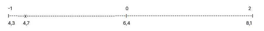
(Physic: 3,2 –> “Physics_G3”: 4,7)
We saw that Michel got a 3,2 in Physic and that qualification is in the Physics_G3 (25% lower grades) with and average math grade of 4,7. We are going to locate this 4,7 grade in the line and do a rule of three to give a theoretical number according the performance of that subject.
The process is simple:
If the group average math grade (x) is lower than the average (6,4):
x = 4,7 (Physics_G3 average)
6,4 – 4,3 = 2,1 (Obtain the length of the range)
4,7 – 4,3 = 0,4 (Obtain the distance from the minim)
(0,4 / 2,1 ) – 1 = -0,8095 (Obtain the value technical value according the range)
If the group average math grade (x) is highier than the average (7,3):
x = 7,3 (Social_studies_G1 average)
8,1 – 6,4 = 1,7 (Obtain the length of the range)
7,3 – 6,4 = 0,9 (Obtain the distance from the average)
(0,9 / 1,7 ) * 2 = 1,0588 (Obtain the value technical value according the range)
If one of the subjects is in the group 4 (the nulls or not enough information) the given value will be 0, so that variable would not have no-impact according to their performance.
- Obtain the final_technical_value
Repeating this process for all the 15 subjects we will obtain 15 values between -1 and 2 according to how they perform in the subjects and how the grades of the subjects are correlated with the grades in maths. Doing the average of all the 15 values we will obtain again a value between -1 and 2, we will call this value the “final_technical_value”. Using the “final_technical_value” we can get a close estimation of Michell’s maths grade. As closer to -1 more likely is that Michel doesn’t get a good grade in maths and as closer to 2 most likely.
What’s more if we use the data of the 200k students to calculate their “final_technical_value” and the maths grade we are going to be able to create confidence intervals. With the intervals we will get a close estimation of the students expected maths grade according the result of the “final_technical_value”.
Benefits:
The main benefit of the RM algorithm is that works well with unstadirsed data. As working with external data sets makes you have no control of the quality of the data and deal with different missing values, executing a ML algorism with a big amount of missing data could cause unexpected results that would impact the performance of the program. Due to the RM algorithm manage well the missing values, making them have a non-impact in the results, makes the algorithm works well with this data sets.
Another positive point of the RM algo is to consider the impact of the worse variables and reward the variables that perform better. During the study of the RM algorism I wanted to remark the importance of the variables that had a bad performance, because is the once I want to avoid, and also give and extra positive point to the best performance variables because are the one I want more. The variables that are at the extremes (-1 and 2) are the once that would impact more and the most relevant once. The evaluation of the variables goes from -1 to the worse and 2 the best, however, there is the same amount of values between (-1, 0) and (0 , 2), this is because I wanted to remark more the best performance variables, due to I am more interested in remark the variables that will maximize the results than penalize the once that perform worse. This means that most values will have a value around 0, and so their performance doesn’t have a considerable impact in the return, and so in the RM algorism.
Why -1 and 2 ?
During the study or creation of this algorithm I tried different limit values to select the best
one. Next, I’m going to explain the different values I tried and why I discard:
– [-1, 1] With this limit range I obtain a distribution where almost all the values where in the
middle, making the most valuable variables don’t have same impact as the final values
selected. So the better performance variables that is what will make our prediction work
better is more likely to have less impact.
– [-2,-1] ^3 – [1, 2]^3: In this case I used the cube exponential, to be able to do exponential
at negative values. The middle values doesn’t affect at the final value because the extremes
have a huge impact due the exponential.
Process explained:
The first step in the training process is to define the variables to study in the RM method. It’s important that all the variables selected has the same format, in our case percentage. Once defined all the variables, the algorism will group each variable in four groups, according to the performance of the variable. The groups will be the next: the variables with the 25% higher performance, the variables with the 25% lowest performance, the variables with average performance (between 25% higher- 25% lower) and the missing or null values. So if for example, the average net income deviation is 1.03% and there is a company with that net income deviation, will be grouped in the group with average performance (between 25%highier- 25%lower), and so if the top 25% higher net income deviation starts at 6% any variable above 6% deviation will be at group 25% higher.
The next step in the process is to discard the variables with non-impact or no relevance, in order to dismiss underrepresented groups that have less than 5% of representation over all the data set. These groups will be considered as a non-relevant variables or null due to there isn’t enough data to work with. With the rest of the variables, the program will calculate the average return for all the groups and add the result in a dictionary with
“VarName_GroupName” as a key and the average return as a value.
Next, the RM algorithm will apply the Range Method to all the variables. The first step in this method is to define the limits and the middle values. The group of variables with the minimum average return of the dictionary will take the value -1, and the max return will take the value 2 and the average will be 0. Once defined all the limits the next point will be to define all the groups between -1 and 2 according to their return. So the variables that perform worse than average will have a negative value and the once better than average will have a positive value between 0 and 2. The null values and the values with less than 5% representation will
automatically have the value 0 assigned so doesn’t affect to the algorism performance. This process is calculated by the next equation:
   if value >= mean_v0:
        y = max_ - mean_v0
        x = value - mean_v0
        technic_value = round(((x / y) * 2), 4)
if value <= mean_v0:
y = value - min_
x = mean_v0 - min_
technic_value = round((( y / x ) - 1), 4)With this equation, all the variables will have the exact value according to their risk o they rentability. The result is going to be added in a dictionary in order to create a function for each variable. The functions will do all the process in the simplest way. Due to I already create the groups and assigned the value to each variable, the function will only create the four groups and return the value assigned in the range method, so the process will be fast and not powering consuming. Once all the functions are created for all the variables, apply this algo
will be as easy as apply all the functions to the daily data and add all the results to obtain the final value. This final value is going to be a technical estimation of how likely the company will maximize the return according to the historical data, being values close to two the most likely and -1 the less likely.
Code:
# Imports:

import pandas as pd
import requests
import seaborn as sns
from pandas_datareader import data
import numpy as np
from sklearn.linear_model import LogisticRegression
from sklearn.model_selection import train_test_split
from sklearn.metrics import r2_score, explained_variance_score, confusion_matrix, accuracy_score, classification_report, log_loss

# Preparete df from the RM method:
## Get data:
df_w_comp = pd.read_csv('file.csv')

## Select companyies to valuate:
columnas_a_grupear = [ 'xxx', 'xxx', 'xxx', 'xxx', 'xxx', 'xxx', 'xxx', 'xxx', 'xxx', 'xxx', 'xxx', 'xxx', 'xxx', 'xxx', 'xxx', 'xxx', 'xxx', 'xxx', 'xxx', 'xxx', 'xxx','xxx', 'xxx', 'xxx', 'xxx', 'xxx', 'xxx', 'xxx', 'xxx', 'xxx', 'xxx', 'xxx', 'xxx', 'xxx', 'xxx',
 'xxx', 'xxx', 'xxx']

## Clean the Target variable:
def clean_df(df):
    df['TV'] = df['TV'].replace(np.nan, 0.000000)
    df = df[df["TV"] != 0.000000]
    df = df.replace(np.nan, 0.000000)
    df.replace([np.inf, -np.inf], 0.000000, inplace=True)
    return df
df_w_comp = clean_df(df_w_comp)


### Funciones group:
def group_of_3(col , lower_25, highier_75 ):

    if (col == 1.000000) or (col == 0.000000):     # --> Avaluate the nan as 0
        return 0
    if (col > highier_75):
        return 3
    if (col < highier_75) and (col > lower_25):
        return 2
    else:
        return 1

all_variances = []
column_values_list = {}

## Create the groups acording the behavoiurs of the variable
name_col_keep = []

for i in columnas_a_grupear:

    try:

        # Get the average value the value 75% and 25% to make the groups

        lower_25 = df_w_comp[i].describe()[4]

        middle = df_w_comp[i].describe()[5]

        highier_75 = df_w_comp[i].describe()[6]

        # New column name of the col grouped
        colum_gr3 = i + "_GR3"
        # Columns grouped:
        name_col_keep.append(colum_gr3)

        # Apply the function to the colum with the values:
        df_w_comp[colum_gr3] = df_w_comp.apply(lambda x: group_of_3(x[i], lower_25,highier_75 ), axis = 1)
        print(df_w_comp.groupby(df_w_comp[colum_gr3]).agg({"TV":["mean", "count"]}))


        # Obtain a list with the results of the target variable in each group:
        # DF with of each column grouped to obtain the average beaviour of the target variable:
        tst = df_w_comp.groupby(df_w_comp[colum_gr3]).agg({"TV":["mean", "count"]})
        #Num of groups
        n = tst.count()[0]

        # Range start from 1 if you don't want to count the group of Nan as a possible max or minim of the  behaviour groups target variable:
        for j in range(1, n):
            #Obtain the beaviour of the target in that group:
            variança = tst.iloc[j]["TV"]["mean"]

            # Add the result to a list :
            all_variances.append(variança)

    except:
        pass


# Get the maxim, min and average values of the list with the average beahviour of each group:
mean_v0 = df_w_comp["variança"].mean()
max_ = max(all_variances)
min_ = min(all_variances)

print("Media -->", mean_v0 )
print("Max -->", max_ )
print("Min -->", min_ )


## Create a dictionary with column and the value:
# For all the columns:
for j in name_col_keep:

    print(j)
    # Count the number of groups:
    tst = df_w_comp.groupby(df_w_comp[j]).agg({"variança":["mean", "count"]})
    n = tst.count()[0]

    #For each group:
    for i in range(0, n):

        # Obtain the Target ratio average and the position of the group:
        variança = tst.iloc[i]["variança"]["mean"]
        print(i)

        # Save the position to be able to get the value by column and position:
        pos = tst.index[i]


        # Avaluative method:

        if variança <= mean_v0:
            y = variança - min_
            x = mean_v0 - min_
            value = round((( y / x ) - 1), 4)


        if variança >= mean_v0:
            y = max_ - mean_v0
            x = variança - mean_v0
            value = round(((x / y) * 2), 4)


        # Create column and position name to save the value:
        column_value_name = j + "_Value_" + str(pos)

        # Save the value:
        column_values_list[column_value_name] = value

        print(variança ," --> " , value )

## Function that avaluate the columns acording the established values
  def value_the_groups(dic, var_name, var_df):

    if (var_df == 0):
        return 0

    if (var_df == 1):
        name_dic_1 =  var_name + "_Value_" + str(1)
        value = dic[name_dic_1]
        return value

    if (var_df == 2):
        name_dic_2 =  var_name + "_Value_" + str(2)
        value = dic[name_dic_2]
        return value

    if (var_df == 3):
        name_dic_3 =  var_name + "_Value_" + str(3)
        value = dic[name_dic_3]
        return value


## Avaluate the columns:
col_avaluades = []
# Apply the values to the groups
col_avaluades = []
for j in name_col_keep:

    print(j ,":")
    print("")

    variable_numered = j + "_Valuated_by_GRp"

    col_avaluades.append(variable_numered)

    try:
        df_w_comp[variable_numered] = df_w_comp.apply(lambda x: value_the_groups(column_values_list, j,  x[j]), axis = 1)

    except:
        pass


# Add the Target to see the results:

TVar= "TV"  # <--- Target var
col_avaluades.append(TVar)
# new df
df_results = df_w_comp[col_avaluades]
# Clean df
df_results = df_results.replace(np.nan, 0)


#Make the operation:

 df_w_comp["final_technical_value"] = (df_w_comp['xxx_GR3_Valuated_by_GRp'] + df_w_comp['xxx_GR3_Valuated_by_GRp'] + df_w_comp['xxx_GR3_Valuated_by_GRp'] + df_w_comp['xxx_GR3_Valuated_by_GRp'] + df_w_comp['growthCommonStock_GR3_Valuated_by_GRp'] + ... + df_w_comp['xxx_GR3_Valuated_by_GRp'])/37

#Results:
g = sns.jointplot(x = df_w_comp["final_technical_value"], y = df_w_comp['TV'], kind='reg')
regline = g.ax_joint.get_lines()[0]
regline.set_color('red')
regline.set_zorder(5)